As you might know already evaluating learning outcomes is very difficult. For example, student feedback is not always reliable; there are studies showing inverse relations between student learning and student ratings (eg. a course that managed to challenge students).
One potential idea is to have the final exam (or even midterms) in the math course written by someone else other than the instructors. Here are some pros:
The instructors’ bias. By having the final exam questions designed by someone else, we substract the frequent issue of (consciously/unconsciously) training the students to pass the final exam. Ultimately the goal of the course is to help the students tackle outside-world challenges using the techniques from the course.
Fitting grades into a bell curve bias. Another frequent issue is being pressured from the department to adjust the test difficulty so that the grades fit the bell curve. So this often leads to unrealistically difficult tests that are less about testing a student’s understanding and more about lowering the average grade.
Smaller percentage grade and instructor performance: The main goal here is to test student learning in an independent way and thus instructor performance. So we can have the final exam grade worth less. We can allow the instructor to spread the grade weight across the learning modules (more quizzes less big tests) to encourage active learning throughout the course.
Here are some cons:
some Course flexibility lost. By “offshoring” the final exam, the course material will have to be suited within some strict guidelines. Meaning that instructors will not be able to test new ideas that they presented during the course.
Too much emphasis on the final exam. This might lead to too much emphasis on the final exam, and less on active learning throughout the course. But that is an existing problem with the current paradigm and if the final exam relative percentage is not too high, that issue can be ameliorated.
“Who will design the final exam?” The main issue here is to have the designer of the exam be independent of the course and that can be hard since the professor faculty is quite small. It might introduce a lot of unnecessary politics. Ideally, the process could be automated using technology (i.e. some algorithmic way of sampling exam questions from a database)
Any feedback, references or anecdotes are welcomed. Do you see any problems with this idea? Is the existing way (exams designed by the instructors) better than what suggested?
Author: thomaskojar
-
Course exams written by someone else other than the instructors/coordinators. Good or Bad?
-
Contour integration
1. Global nature
An important feature to note about Cauchy’s theorem is the global nature of its hypothesis on the analytic functions f. Cauchy’s theorem is the powerful technique of contour shifting, which allows one to compute a contour integral by replacing the contour with a homotopic contour on which the integral is easier to either compute or integrate.
2. Rigidity for non-analytic
3. Analyticity criterion: Morera’s theorem
4. Cauchy’s theorem, Poisson Kernel and Brownian motion
For $latex |z|<1$ and $\theta$ real define the Cauchy kernel by
$latex C(\theta,z):=\frac{1}{2\pi}\ \frac{e^{i\theta}}{e^{i\theta}-z}\quad,$
and define the Cauchy transform of a continuous function $latex g$ on the unit circle $latex \partial D$ by
$latex (Cg)(z):=\int_0^{2\pi}g(e^{i\theta})\ C(\theta,z)\ d\theta$
for $latex |z|<1$. In particular Cauchy’s Formula says that if $latex g$ is the boundary value of a holomorphic function $latex f$ on $latex D$, then $latex Cg=f$.
-
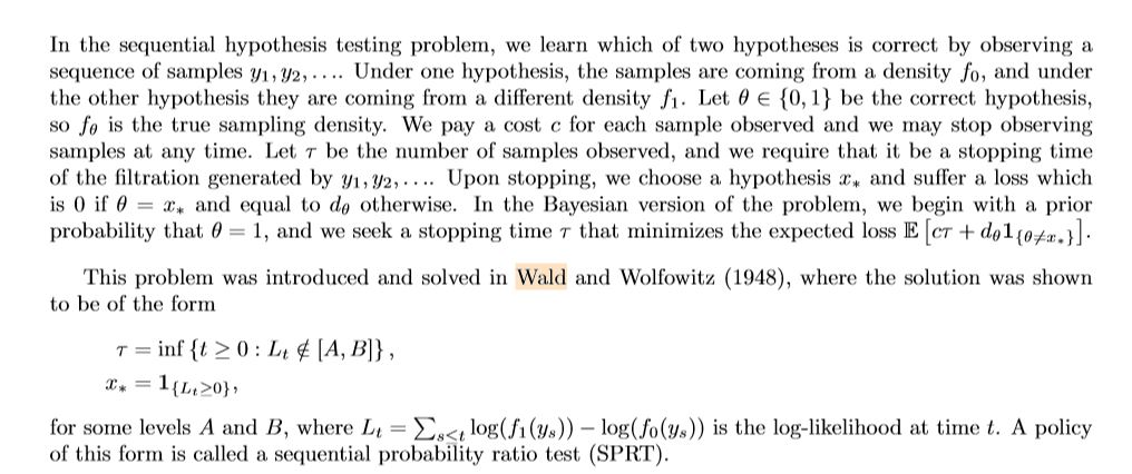
Wald’s equation and bullet projectile quality
References: Milton Friedman suggesting problem to Wald and the math in sequential analysis.
In order to understand the story, it is necessary to have an idea of a simple statistical problem, and of the standard procedure for dealing with it. The actual problem out of which sequential analysis grew will serve. The Navy has two alternative designs (say A and B) for a projectile. It wants to determine which is superior. To do so it undertakes a series of paired firings. On each round, it assigns the value 1 or 0 to A accordingly as its performance is superior or inferior to that of B and conversely 0 or 1 to B. The Navy asks the statistician how to conduct the test and how to analyze the results.
The standard statistical answer was to specify a number of firings (say 1,000) and a pair of percentages (e.g., 53% and 47%) and tell the client that if A receives a 1 in more than 53% of the firings, it can be regarded as superior; if it receives a 1 in fewer than 47%, B can be regarded as superior; if the percentage is between 47% and 53%, neither can be so regarded.
When Allen Wallis was discussing such a problem with (Navy) Captain Garret L. Schyler, the captain objected that such a test, to quote from Allen’s account, may prove wasteful. If a wise and seasoned ordnance officer like Schyler were on the premises, he would see after the first few thousand or even few hundred [rounds] that the experiment need not be completed either because the new method is obviously inferior or because it is obviously superior beyond what was hoped for.
-
Zero level set of 2D NSE
Conformal invariance (CI)
In “Conformal invariance in two-dimensional turbulence” by Bernard etal, it was guessed that numerically the zero level set (ZLS) for the vorticity field has the same properties as an SLE curve.
- Since NSE and Euler equations are volume preserving, the equations themselves are not conformally invariant. So one has to study the equations satisfied by the countour lines themselves.
- The zero level set is in the intersection of the support of all invariant measures. Recall that this holds, because there is a small probability that the random forces are close to zero for any given time interval so the fluid flow slows down due to viscosity. Moreover, the invariant measures seem to possess strong scale invariance properties, at least in the inverse cascade regime. So the zero level set has some special statistical properties that other level sets do not.
- Since the linearization is stochastic heat equation (SHE) whose stationary solution is the Gaussian free field (GFF), it is reasonable that in the long run the ZLS of 2DNSE is close to the ZLS of SHE which is in turn close to the ZLS of GFF aka SLE(4).
Dimension of the zero level set
What is the dimension of zero vorticity level set?
-
Periodic TASEP
KPZ Fixed point
-
- Finding a transition probability formula that is amenable to taking limit as the number of TASEP particles goes to infinity.
- Is there an analogous backwards heat equation problem as in the KPZ fixed point for Z-TASEP?
- Identifying the KPZ fixed point in the subcritical region
- Finding a transition probability formula that is amenable to taking limit as the number of TASEP particles goes to infinity.
.
RSK correspondence formula
In “Determinantal transition kernels for some interacting particles on the line” Dieker and Warren derive the transition probability formula for various particle processes on the infinite line. For example, they rederived Schutz’s formula for Z-TASEP. Can the Baik-Liu formula be rederived in the same spirit of techniques.
- What will be the periodic Gelfand-Tsetlin and Young Tableaus that are in bijection with the dynamics of periodic TASEP?
-
-
Elliptic divergence operator isomorphism for Lp spaces p greater than 2
For the problem $latex Lu:=div(A\nabla u)=div(g)$, we will show $latex L: W_{0}^{1,p}\to W^{-1,p} $ (cf. Meyers “An Lp-estimate for the gradient of solutions of second order elliptic divergence equations “). Assume that we have coercivity: $latex \inf_{\phi\in L^{1/q’}}\sup_{\psi\in L^{1/q}}|B_{A}(\psi,\phi) |\geq \frac{1}{K}> 0$.
- Suppose that $latex g\in L^{q’}$ and consider sequence $latex g_{k}\in L^{2}$ such that $latex |g_{k}-g|_{L^{q’}}\to 0$.
- For $latex div(A\nabla u_{k})=div(g_{k})$ the solutions $latex u_{k}\in W^{1,2}_{0}$. From the coercivity assumption we get: $latex | \nabla u_k |_{q’}\leq K| g_k |_{q’}$.
- Therefore, there exists $latex u\in W^{1,q’}$ s.t. $latex \nabla u_{k}\to \nabla u$ weakly in $latex L^{q’}$.
- Therefore, u solves the original problem $latex B_{A}(\psi, u)-\int_{\Omega} (\nabla \psi, g)dx=B_{A}(\psi, u-u_{k})+\int_{\Omega} (\nabla \psi, g_{k}-g)dx\to 0$.
- and satisfies the estimate $latex |\nabla u |_{q’}\leq K |g |_{q’}$.
-
Proofs of CLT
Proofs of Central limit theorem
- Method of characteristics
http://www.cs.toronto.edu/~yuvalf/CLT.pdf
- Method of Moments
http://www.cs.toronto.edu/~yuvalf/CLT.pdf
- Minimizing Entropy
“An information-theoretic proof of the central limit theorem with the Lindeberg condition” - Heat equation
Kolmogorov Petrovsky - Stein’s method
https://normaldeviate.wordpress.com/2013/11/16/steins-method/
- Method of characteristics